Analytics

Here is a tutorial on Google Colab that shows how to use the analytics module

Probing

class labml.analytics.ModelProbe(model: nn.Module, name: str = 'model', *, add_forward_hooks=True, add_backward_hooks=False)

You can wrap any PyTorch model with ModelProbe to access it’s parameters, activations and gradients.

Here’s a notebook with example usage

>>> from labml.analytics import ModelProbe
>>> probe = ModelProbe(model)
>>> outputs = model(inputs)
>>> outputs.backward()
>>> probe.forward_output["*attention*"].get_dict()
>>> probe.parameters['*.bias'].get_list()

property parameters

All the model parameters as a ValueCollection

property forward_input

Inputs to layers in the forward pass as a ValueCollection

property forward_output

Outputs of layers in the forward pass as a ValueCollection

property backward_input

Inputs (gradients) to layers in the backward pass as a ValueCollection

property backward_output

Output (gradients) of layers in the backward pass as a ValueCollection

class labml.analytics.ValueCollection(values: Dict[str, any], keys: List[str])

get_value(key: str)

Get a value by key

Parameters

key (str) – Key of the value

get_list()

Get a list of values

get_dict()

Get a dictionary of values

deep()

Get a DeepValueCollection by expanding the tree of values

class labml.analytics.DeepValueCollection(values: Dict[str, any], keys: List[str])

get_value(key: str)

Get a value by key. Use / to go navigate into child elements.

Parameters

key (str) – Key of the value

get_list()

Get a list of values

get_dict()

Get a dictionary of values

Get data

labml.analytics.runs(*uuids: str)

This is used to analyze runs. It fetches all the log indicators.

Parameters

uuids (str) – UUIDs of the runs. You can get this from labml.ai app

Example

>>> from labml import analytics
>>> indicators = analytics.runs('1d3f855874d811eabb9359457a24edc8')

labml.analytics.get_run(uuid: str)

Returns Run object

labml.analytics.set_preferred_db(db: str)

Set the preference to load data from.

Parameters

db (str) – Either tensorboard or sqlite

labml.analytics.indicator_data(indicators: IndicatorCollection) → Tuple[List[ndarray], List[List[str]]]

Returns a tuple of a list of series and a list of names of series. Each series, S is a timeseries of histograms of shape [T, 10], where T is the number of timesteps. S[:, 0] is the global_step. S[:, 1:10] represents the distribution at basis points 0, 6.68, 15.87, 30.85, 50.00, 69.15, 84.13, 93.32, 100.00.

Example

>>> from labml import analytics
>>> indicators = analytics.runs('1d3f855874d811eabb9359457a24edc8')
>>> analytics.indicator_data(indicators)

labml.analytics.artifact_data(indicators: IndicatorCollection) → Tuple[List[any], List[str]]

Returns a tuple of a list of series and a list of names of series. Each series, S is a timeseries of histograms of shape [T, 10], where T is the number of timesteps. S[:, 0] is the global_step. S[:, 1:10] represents the distribution at basis points: 0, 6.68, 15.87, 30.85, 50.00, 69.15, 84.13, 93.32, 100.00.

Example

>>> from labml import analytics
>>> indicators = analytics.runs('1d3f855874d811eabb9359457a24edc8')
>>> analytics.artifact_data(indicators)

class labml.analytics.IndicatorCollection(indicators: List[Indicator])

You can get a indicator collection with runs().

>>> from labml import analytics
>>> indicators = analytics.runs('1d3f855874d811eabb9359457a24edc8')

You can reference individual indicators as attributes.

>>> train_loss = indicators.train_loss

You can add multiple indicator collections

>>> losses = indicators.train_loss + indicators.validation_loss

Plot

labml.analytics.distribution(indicators: IndicatorCollection, *, names: Optional[List[str]] = None, levels: int = 5, alpha: int = 0.6, color_scheme: str = 'tableau10', height: int = 400, width: int = 800, height_minimap: int = 100)

labml.analytics.distribution(series: List[Union[ndarray, torch.Tensor]], *, names: Optional[List[str]] = None, levels: int = 5, alpha: int = 0.6, color_scheme: str = 'tableau10', height: int = 400, width: int = 800, height_minimap: int = 100)

labml.analytics.distribution(series: List[Union[ndarray, torch.Tensor]], step: ndarray, *, names: Optional[List[str]] = None, levels: int = 5, alpha: int = 0.6, color_scheme: str = 'tableau10', height: int = 400, width: int = 800, height_minimap: int = 100)

labml.analytics.distribution(series: Union[ndarray, torch.Tensor], *, names: Optional[List[str]] = None, levels: int = 5, alpha: int = 0.6, color_scheme: str = 'tableau10', height: int = 400, width: int = 800, height_minimap: int = 100)

Creates a distribution plot distribution with Altair

This has multiple overloads

labml.analytics.distribution(indicators: IndicatorCollection, *, names: Optional[List[str]] = None, levels: int = 5, alpha: int = 0.6, height: int = 400, width: int = 800, height_minimap: int = 100)

labml.analytics.distribution(series: Union[np.ndarray, torch.Tensor], *, names: Optional[List[str]] = None, levels: int = 5, alpha: int = 0.6, height: int = 400, width: int = 800, height_minimap: int = 100)

labml.analytics.distribution(series: List[Union[np.ndarray, torch.Tensor]], *, names: Optional[List[str]] = None, levels: int = 5, alpha: int = 0.6, height: int = 400, width: int = 800, height_minimap: int = 100)

labml.analytics.distribution(series: List[Union[np.ndarray, torch.Tensor]], step: np.ndarray, *, names: Optional[List[str]] = None, levels: int = 5, alpha: int = 0.6, height: int = 400, width: int = 800, height_minimap: int = 100)

Parameters

• indicators (IndicatorCollection) – Set of indicators to be plotted

• series (List[np.ndarray]) – List of series of data

• step (np.ndarray) – Steps

Keyword Arguments

• names (List[str]) – List of names of series

• levels – how many levels of the distribution to be plotted

• alpha – opacity of the distribution

• color_scheme – color scheme

• height – height of the visualization

• width – width of the visualization

• height_minimap – height of the view finder

Returns

The Altair visualization

Example

>>> from labml import analytics
>>> indicators = analytics.runs('1d3f855874d811eabb9359457a24edc8')
>>> analytics.distribution(indicators)

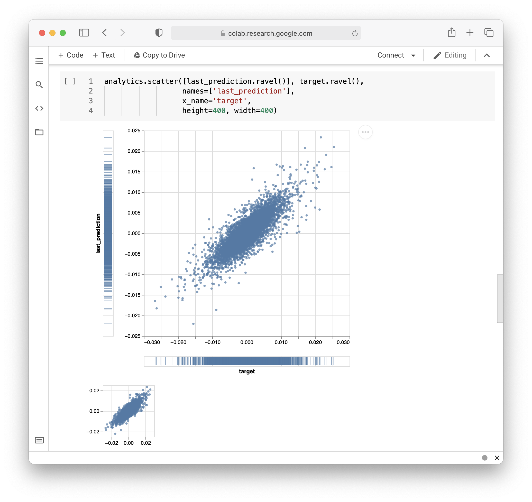
labml.analytics.scatter(indicators: IndicatorCollection, x_indicators: IndicatorCollection, *, names: Optional[List[str]] = None, x_name: Optional[str] = None, noise: Optional[Tuple[float, float]] = None, circle_size: int = 20, height: int = 400, width: int = 800, height_minimap: int = 100)

labml.analytics.scatter(series: List[ndarray], x_series: ndarray, *, names: Optional[List[str]] = None, x_name: Optional[str] = None, noise: Optional[Tuple[float, float]] = None, circle_size: int = 20, height: int = 400, width: int = 800, height_minimap: int = 100)

Creates a scatter plot with Altair

This has multiple overloads

labml.analytics.scatter(indicators: IndicatorCollection, x_indicators: IndicatorCollection, *, names: Optional[List[str]] = None, x_name: Optional[str] = None, noise: Optional[Tuple[float, float]] = None, circle_size: int = 20, height: int = 400, width: int = 800, height_minimap: int = 100)

labml.analytics.scatter(series: List[np.ndarray], x_series: np.ndarray, *, names: Optional[List[str]] = None, x_name: Optional[str] = None, noise: Optional[Tuple[float, float]] = None, circle_size: int = 20, height: int = 400, width: int = 800, height_minimap: int = 100)

Parameters

• indicators (IndicatorCollection) – Set of indicators to be plotted

• x_indicators (IndicatorCollection) – Indicator for x-axis

• series (List[np.ndarray]) – List of series of data

• x_series (np.ndarray) – X series of data

Keyword Arguments

• names (List[str]) – List of names of series

• name (str) – Name of X series

• noise – Noise to be added to spread out the scatter plot

• circle_size – size of circles in the plot

• height – height of the visualization

• width – width of the visualization

• height_minimap – height of the view finder

Returns

The Altair visualization

Example

>>> from labml import analytics
>>> indicators = analytics.runs('1d3f855874d811eabb9359457a24edc8')
>>> analytics.scatter(indicators.validation_loss, indicators.train_loss)

labml.analytics.binned_heatmap(indicators: IndicatorCollection, x_indicators: IndicatorCollection, *, names: Optional[List[str]] = None, x_name: Optional[str] = None, height: int = 400, width: int = 800, height_minimap: int = 100)

labml.analytics.binned_heatmap(series: List[ndarray], x_series: ndarray, *, names: Optional[List[str]] = None, x_name: Optional[str] = None, height: int = 400, width: int = 800, height_minimap: int = 100)

Creates a scatter plot with Altair

This has multiple overloads

labml.analytics.binned_heatmap(indicators: IndicatorCollection, x_indicators: IndicatorCollection, *, names: Optional[List[str]] = None, x_name: Optional[str] = None, height: int = 400, width: int = 800, height_minimap: int = 100)

labml.analytics.binned_heatmap(series: List[np.ndarray], x_series: np.ndarray, *, names: Optional[List[str]] = None, x_name: Optional[str] = None, height: int = 400, width: int = 800, height_minimap: int = 100)

Parameters

• indicators (IndicatorCollection) – Set of indicators to be plotted

• x_indicators (IndicatorCollection) – Indicator for x-axis

• series (List[np.ndarray]) – List of series of data

• x_series (np.ndarray) – X series of data

Keyword Arguments

• names (List[str]) – List of names of series

• name (str) – Name of X series

• noise – Noise to be added to spread out the scatter plot

• circle_size – size of circles in the plot

• height – height of the visualization

• width – width of the visualization

• height_minimap – height of the view finder

Returns

The Altair visualization

Example

>>> from labml import analytics
>>> indicators = analytics.runs('1d3f855874d811eabb9359457a24edc8')
>>> analytics.scatter(indicators.validation_loss, indicators.train_loss)

labml.analytics.histogram(series: Union[ndarray, torch.Tensor], *, low: Optional[float] = None, high: Optional[float] = None, height: int = 400, width: int = 800, height_minimap: int = 100)

Creates a histogram with Altair

Parameters

series (Union[np.ndarray, torch.Tensor]) – Data

Keyword Arguments

• low – values less than this are ignored

• high – values greater than this are ignored

• height – height of the visualization

• width – width of the visualization

• height_minimap – height of the view finder

Returns

The Altair visualization